Optimization : Boltzmann Machines & Deep Belief Nets

As we have already talked about the evolution of Neural nets in our previous posts, we know that since their inception in 1970’s, these Networks have revolutionized the domain of Pattern Recognition.

The Networks developed in 1970’s were able to simulate a very limited number of neurons at any given time, and were therefore not able to recognize patterns involving higher complexity.
However, by the end of  mid 1980’s these networks could simulate many layers of neurons, with some serious limitations – that involved human involvement (like labeling of data before giving it as input to the network & computation power limitations ). This was possible because of Deep Models developed by Geoffery Hinton. 
Hinton in 2006, revolutionized the world of deep learning with his famous paper ” A fast learning algorithm for deep belief nets ”  which provided a practical and efficient way to train Supervised deep neural networks.

In 1985 Hinton along with Terry Sejnowski invented an Unsupervised Deep Learning model, named Boltzmann Machine. These are Stochastic (Non-Deterministic) learning processes having recurrent structure and are the basis of the early optimization techniques used in ANN; also known as Generative Deep Learning model which only has Visible (Input) and Hidden nodes.

OBJECTIVE

Boltzmann machines are designed to optimize the solution of any given problem, they optimize the weights and quantity related to that particular problem.

It is of importance to note that Boltzmann machines have no Output node and it is different from previously known Networks (Artificial/ Convolution/Recurrent), in a way that its Input nodes are interconnected to each other.

The below diagram shows the Architecture of a Boltzmann Network:

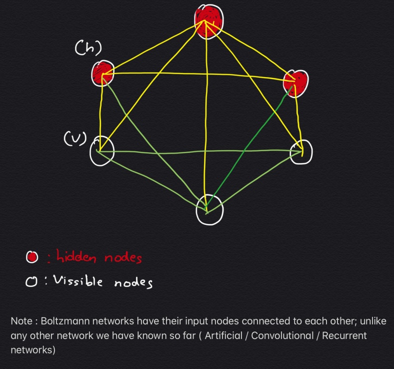
All these nodes exchange information among themselves and self-generate subsequent data, hence these networks are also termed as Generative deep model.

These Networks have 3 visible nodes (what we measure) & 3 hidden nodes (those we don’t measure); boltzmann machines are termed as Unsupervised Learning models because their nodes learn all parameters, their patterns and correlation between the data, from the Input provided and forms an Efficient system. This model then gets ready to monitor and study abnormal behavior depending on what it has learnt.
This model is also often considered as a counterpart of Hopfield Network, which are composed of binary threshold units with recurrent connections between them.

Types of Boltzmann Machines

  • EBM ( Energy Based models )
  • RBM (Restricted Boltzmann Machines )


Energy – Based Models

EBMs can be thought as an alternative to Probabilistic Estimation for problems such as prediction, classification, or other decision making tasks, as their is no requirement for normalisation.

Formula for Boltzmann Distribution

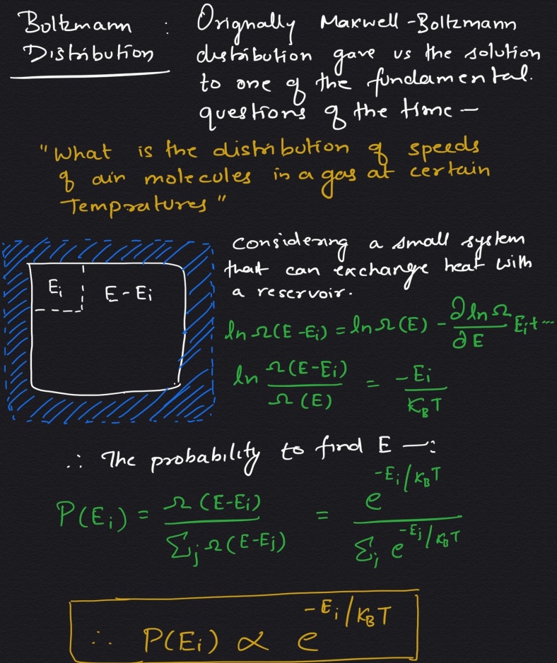
This equation is used for sampling distribution memory for Boltzmann machines, here,  P stands for Probabilityfor Energy (in respective states, like Open or Closed), T stands for Timek: boltzmann constantTherefore for any system at temperature T, the probability of a state with energy, E is given by the above distribution.
Note: Higher the energy of the state, lower the probability for it to exist.

In the statistical realm and Artificial Neural Nets, Energy is defined through the weights of the synapses, and once the system is trained with set weights(W), then system keeps on searching for lowest energy state for itself by self-adjusting.
These EBMs are sub divided into 3 categories:

  • Linear Graph Based Models ( CRF / CVMM / MMMN )
  • Non-Linear Graph Based models
  • Hierarchical Graph based models

Conditional Random Fields (CRF) use a negative log-likelihood loss function to train linear structured models.
Max-Margin Markov Networks(MMMN) uses Margin loss to train linearly parametrized factor graph with energy func- optimised using SGD.

Training/ Learning in EBMs 

The fundamental question that we need to answer here is ” how many energies of incorrect answers must be pulled up before energy surface takes the right shape.
Probabilistic learning is a special case of  energy based learning where loss function is negative-log-likelihood. The negative log-likelihood loss pulls up on all incorrect answers at each iteration, including those that are unlikely to produce a lower energy than the correct answer. Therefore optimizing the loss function with SGD is more efficient than black-box convex optimization methods; also because it can be applied to any loss function- local minima is rarely a problem in practice because of high dimensionality of the space.

Restricted Boltzmann Machines & Deep Belief Nets

Shifting our focus back to the original topic of discussion ie
Deep Belief Nets, we start by discussing about the fundamental blocks of a deep Belief Net ie RBMs ( Restricted Boltzmann Machines ).

As Full Boltzmann machines are difficult to implement we keep our focus on the Restricted Boltzmann machines that have just one minor but quite a significant difference – Visible nodes are not interconnected – .
RBM 
algorithm is useful for dimensionality reduction, classification, Regression, Collaborative filtering, feature learning & topic modelling.

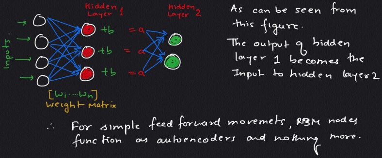
The important question to ask here is how these machines reconstruct data by themselves in an unsupervised fashion making several forward and backward passes between visible layer and hidden layer 1, without involving any further deeper network.

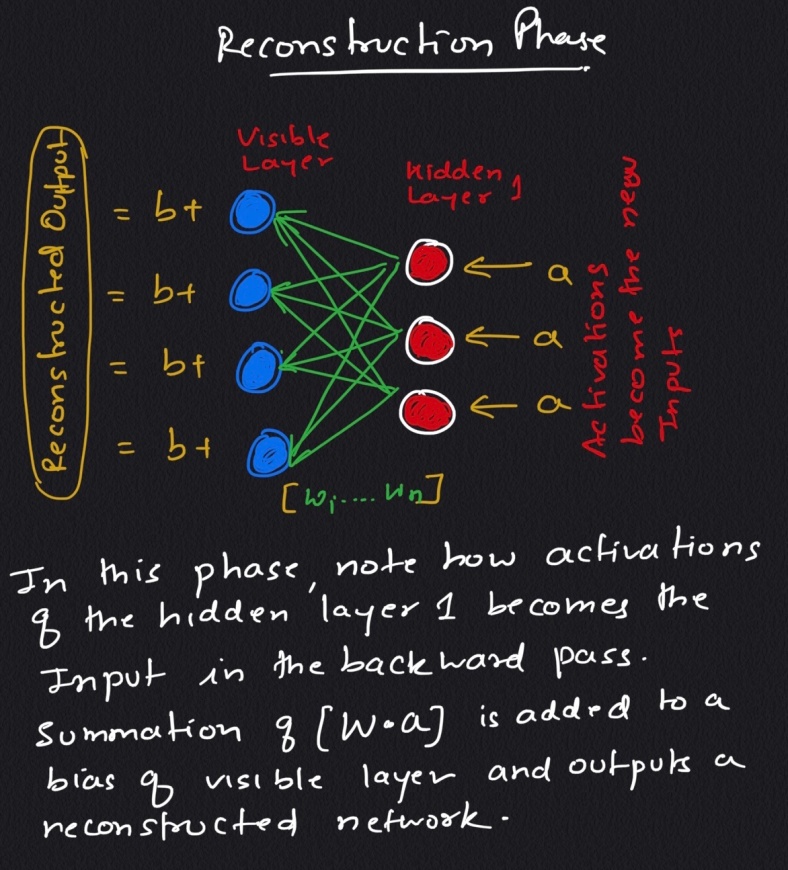
note : the output shown in the above figure is an approximation of the original Input.
Since the weights are randomly initialized, the difference between Reconstruction and Original input is Large.

It can be observed that, on its forward pass, an RBM uses inputs to make predictions about node activation, or the probability of output given a weighted x: p(a|x; w). But on its backward pass, when activations are fed in and reconstructions of the original data, are spit out, an RBM is attempting to estimate the probability of inputs x given activations a, which are weighted with the same coefficients as those used on the forward pass. This second phase can be expressed as p(x|a; w). Together giving the joint probability distribution of x and activation a .

Reconstruction is making guesses about the probability distribution of the original input; i.e. the values of many varied points at once. This is known as generative learning, and this must be distinguished from discriminative learning performed by classification, ie mapping inputs to labels.

Conclusions & Next Steps

You can interpret RBMs’ output numbers as percentages. Every time the number in the reconstruction is not zero, that’s a good indication the RBM learned the input.

It should be noted that RBMs do not produce the most stable, consistent results of all shallow, feedforward networks. In many situations, a dense-layer autoencoder works better. Indeed, the industry is moving toward tools such as variational autoencoders and GANs.

Training YOLO v3 on custom Data set on Linux

YOLOs orignal concept is to be credited to Joseph Redmon, Ross Girshick, Santosh Divvala, Ali Farhadi.

Prerequisite:

1. Setup CUDA and cuDNN on your system, follow here (requires GPU, Ignore this step if you have a Only CPU machine)
2. Have all the libraries installed as per your knowledge, anything missing can be installed later.
NOTE : If you are using a Windows System to start using Darknet you must have a ‘GCC compiler’ and Linux like ‘make’ command.
Solution : Install Cygwin, and under DEVEL search, look for “gcc, make” and install

Download Darknet Code of YOLO from : https://github.com/pjreddie/darknet
Download YOLOv3 Weights file here: https://pjreddie.com/media/files/yolov3.weights
Download YOLOv2 weights file here: https://pjreddie.com/media/files/yolo.weights
Download darknet-53 weights file : https://pjreddie.com/media/files/darknet53.conv.74

  • we use these weight files for Transfer Learning, you can definitely train your model from scratch if you want, for that you may not require these weight files
  • place these weight files inside the “darknet-master” folder.

$ git clone https://github.com/pjreddie/darknet
$ cd darknet
If you wish to train the model for your own dataset using the GPU.
* open ‘Makefile’ and Change the GPU 0 to 1 and save it. If you installed openCV set OPENCV 0 to 1 otherwise not need.
$ make ( ‘make’ command compiles the darknet code)

How to make predictions on a Test Image using the pre-trained model of Darknet

To check you have got the darknet working , type : $ ./darknet
Expected Output >
usage: ./darknet <function>

Running darknet testing on a dog.jpg present data folder

Note: config file of Yolov3 is present in cfg folder; weight file is present in the root directory of ie the ‘darknetmaster‘ folder; test data is in data folder with name “dog.jpg”.

Just in case you guys get an error of “Aborted (Core Dump)” or “CUDA error : Out of Memory” like the one below, do the following :

Solution
1. open the cfg / yolov3.cfg
2. remove ‘#’ from Line 3 and Line 4 under ‘Testing” section

i.e #batch=1 ——————-> batch=1 and
#subdivisions=1 —————> subdivisions=1

Annotation & Data prepration

  1. Data Annotation : Create .txt-file for each .jpg-image-file – in the same directory and with the same name.
    Here is an example below for creating the txt file for each image.

Using LabelImg an Annotation tool , saves the annotation in YOLO format already, so you may get the txt in the above mentioned format.
LabelImg can be downloaded from here : https://github.com/tzutalin/labelImg.git

NOTE : To train with a YOLO configuration , you MUST have annotation in the above mentioned format.
Write a script if you have to, and get the txt in above format

2. Next step involves separating Training data & Testing data.
For this use the following code :
< please insert the path of dataset with annotation file in Line 5 >

import glob, os
# Current directory 
current_dir = os.path.dirname(os.path.abspath(__file__))
print(current_dir)
current_dir = '<Your Dataset Path>' 
# Percentage of images to be used for the test set 
percentage_test = 10;
# Create and/or truncate train.txt and test.txt 
file_train = open('train.txt', 'w') 
file_test = open('test.txt', 'w')
# Populate train.txt and test.txt
counter = 1 
index_test = round(100 / percentage_test)
for pathAndFilename in glob.iglob(os.path.join(current_dir, "*.jpg")):  
    title, ext = os.path.splitext(os.path.basename(pathAndFilename))
    if counter == index_test:
        counter = 1
        file_test.write(current_dir + "/" + title + '.jpg' + "\n")
    else:
        file_train.write(current_dir + "/" + title + '.jpg' + "\n")
        counter = counter + 1

Preparing the configuration file YOLOv3

Prerequisites :

  • Download a simple sample dataset with just 1 class from here

YOLO versions require 3 types of files to run training with them:

a) backup/customdata.names : this file contains the names of classes. Every new category should be on a new line, its line number should match the category number in the .txt label files we created earlier.
Since we have just 1 class

NFPA

b) backup/customdata.data : this file contains the following data:

  • no of classes we are training our data on
  • Training data list inside (train.txt), Testing data list inside (test.txt) ie path of jpg files that have been annotated
  • File that contains the names for the categories
  • Location where weight files must be saved
classes = 1
train = /home/ankit/Downloads/ImgLearning/darknet/backup/train.txt
valid = /home/ankit/Downloads/ImgLearning/darknet/backup/test.txt 
names = /home/ankit/Downloads/ImgLearning/darknet/backup/<coustomddata>.names
backup = /home/ankit/Downloads/ImgLearning/darknet/backup/

c) cfg/’customdata’.cfg

Following changes must be made inside the cfg file based on the 
number of classes you want to train your model on: (our case class=1)

Line 603 : set filters = (classes + 5)*3 in our case filters = 18
Line 610 : set classes = 1, i.e the number of category we want to detect
Line 689 : set filters = (classes + 5)*3 in our case filters = 18 Line 696 : set classes = 1, i.e the number of category we want to detect Line 776 : set filters = (classes + 5)*3 in our case filters = 18 Line 783 : set classes = 1, i.e the number of categories we want to detect

If you would have paid attention to the above line numbers of yolov3.cfg, you would observe that these changes are made to YOLO layers of the network and the layer just prior to it!

Now, Let the training begin!!

$ ./darknet detector train backup/nfpa.data cfg/yolov3.cfg weights/darknet53.conv.74


Nitty-Witty of YOLO v3

Modify code to save weight files regularly

Locate the file detector.c and change the line #135 (probably) from:

if(i%10000==0 || (i < 1000 && i%100 == 0)){ to
if(i%1000==0 || (i < 2000 && i%200 == 0)){

The original upper line saves the network weights after every 100 iterations till first 1000 and then saves only after every 10000 iterations. In the below case, we save after every 200 iterations till we reach 2000 and then we save after every 1000 iterations.
After the above changes are made, we need to recompile using the “make” command.

Hyperparameters

batch=64  ''' It is impractical to (and unnecessary) to use 
all images in the training set at once to update the weights.
So, a small subset of images is used in one iteration, and this 
subset is called the batch size.'''
subdivisions=16 ''' it refers to the fraction of batch size that
 will be processed on the GPU in one go
You can start the training with subdivisions=1,  
and if you get < out of memory> error, increase these subdivisions by multiple of 2 (eg 2,4,8,16) till the training proceeds successfully
The GPU processes batch/subdivisions number of images at any time, but full batch iteration completes only after all images are processed 

NOTE : During testing, both batch and subdivision are set to 1.
width=608    ''' it is the size to which original image will be resized 
height=608       before the training begins. ''' 
channels=3       Channel shows we will use RGB image
momentum=0.9   to penalise large weight changes between iterations
decay=0.0005   to penalise wights in case of Over-fitting
max_batches = 500200  No of Iterations training must run for

To save terminal logs and Plot Loss from it

The below command will save all the training logs visible on terminal into a <.log> file for future reference.

To save the Logs use below command
$ ./darknet detector train backup/nfpa.data cfg/yolov3.cfg weights/darknet53.conv.74 >> backup/<name>.log

To plot the loss from above saved log file
$ python3 plot_logfile_loss.py backup/<name>.log


Network Loading fails while Training using Pre-trained weights?

I have sometimes encountered the problem that my network wouldn’t load and ends with (ABORT) error if I use a pre-trained weights, but the training starts if the pre-trained weight is removed.
My best guess to this problem is the weight file is corrupted at some level hence change or download again the weight file.

Want to play with the layers of YOLO and modify its Architecture?

Good thing about Darknet Yolo is that its complete architecture is inside the “.cfg” file and therefore it is not required to mess around the the code to change its architecture.

Open the respective cfg file you are working on identify the layer you wish to modify and make the required modification, simply try by deleting the last layer, and see if the change is visible on your terminal when the network is being loaded.

Want to generate custom Anchor boxes for your data set ?

Use the python script “anchor_box_generator.py” from my Github repository available in the following link .

Table detection file